23  Analysis of simulation results

library(ggplot2)
library(readr)

experiments_path <- "assets/netlogo/experiments/Artificial Anasazi_experiments "

color_mapping <- c("historical households" = "blue", 
                   "simulation households" = "darkred")

23.1 Single run

expname <- "experiment single run"

Read output:

results_single <- readr::read_csv(paste0(experiments_path, expname, "-table.csv"), skip = 6)

Rows: 552 Columns: 11
── Column specification ────────────────────────────────────────────────────────
Delimiter: ","
chr (1): map-view
dbl (9): [run number], fertility, death-age, harvest-variance, fertility-end...
lgl (1): historic-view?

ℹ Use `spec()` to retrieve the full column specification for this data.
ℹ Specify the column types or set `show_col_types = FALSE` to quiet this message.

Plot trajectories of metrics:

plot_name <- paste0(experiments_path, expname, "-trajectories.png")

png(plot_name, width = 840, height = 540)

ggplot(results_single) +  
  geom_line(aes(x = `[step]`, y = `historical-total-households`, color = "historical data"),
            linewidth = 1.2) +
  geom_line(aes(x = `[step]`, y = `total-households`, color = "simulation households"),
            linewidth = 1.2) +
  labs(x = "steps", y = "households") +
  scale_color_manual(name = "", values = color_mapping) +
  theme(legend.position = "right")

dev.off()

svg 
  2 

knitr::include_graphics(plot_name)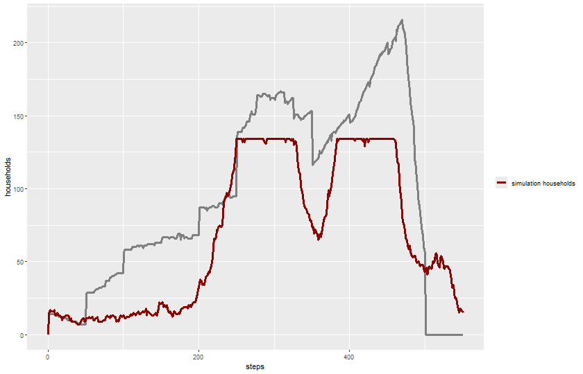

23.2 Multiple runs in single configuration

expname <- "experiment multiple runs"

Read output:

results_single <- readr::read_csv(paste0(experiments_path, expname, "-table.csv"), skip = 6)

Rows: 5520 Columns: 11
── Column specification ────────────────────────────────────────────────────────
Delimiter: ","
chr (1): map-view
dbl (9): [run number], fertility, death-age, harvest-variance, fertility-end...
lgl (1): historic-view?

ℹ Use `spec()` to retrieve the full column specification for this data.
ℹ Specify the column types or set `show_col_types = FALSE` to quiet this message.

Plot trajectories of metrics:

plot_name <- paste0(experiments_path, expname, "-trajectories.png")

png(plot_name, width = 840, height = 540)

ggplot(results_single) +  
  geom_line(aes(x = `[step]`, y = `total-households`, color = `[run number]`, group = `[run number]`),
            linewidth = 1.2) +
  geom_line(aes(x = `[step]`, y = `historical-total-households`), 
            color = color_mapping["historical households"],
            linewidth = 1.2, linetype = 2) +
  labs(x = "steps", y = "households") +
  theme(legend.position = "right")

dev.off()

svg 
  2 

knitr::include_graphics(plot_name)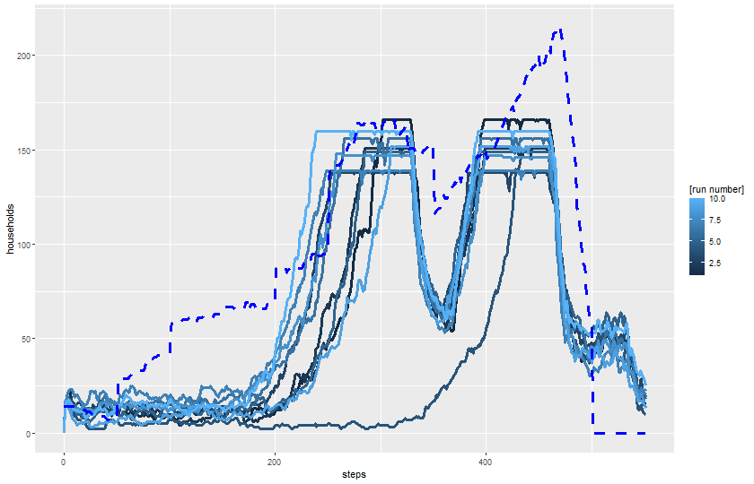

23.3 Parameter exploration - regular intervals

23.3.1 One parameter

expname <- "experiment harvest adjustment"

Read output:

results_harvest_adj <- readr::read_csv(paste0(experiments_path, expname, "-table.csv"), skip = 6)

Rows: 104880 Columns: 11
── Column specification ────────────────────────────────────────────────────────
Delimiter: ","
chr (1): map-view
dbl (9): [run number], fertility, death-age, harvest-variance, fertility-end...
lgl (1): historic-view?

ℹ Use `spec()` to retrieve the full column specification for this data.
ℹ Specify the column types or set `show_col_types = FALSE` to quiet this message.

Plot trajectories of metrics:

plot_name <- paste0(experiments_path, expname, "-trajectories.png")

png(plot_name, width = 840, height = 540)

ggplot(results_harvest_adj) +  
  geom_line(aes(x = `[step]`, y = `total-households`, color = `harvest-adjustment`, group = `[run number]`),
            linewidth = 1.2) +
  geom_line(aes(x = `[step]`, y = `historical-total-households`), color = "black",
            linewidth = 1.2, linetype = 2) +
  labs(x = "steps", y = "households") +
  theme(legend.position = "right")

dev.off()

svg 
  2 

knitr::include_graphics(plot_name)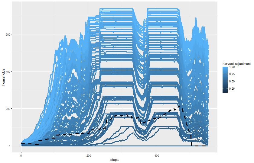

23.3.2 Two parameter

expname <- "experiment harvest adjustment variance"

Read output:

results_harvest_adj <- readr::read_csv(paste0(experiments_path, expname, "-table.csv"), skip = 6)

Rows: 441600 Columns: 11
── Column specification ────────────────────────────────────────────────────────
Delimiter: ","
chr (1): map-view
dbl (9): [run number], fertility, death-age, harvest-variance, fertility-end...
lgl (1): historic-view?

ℹ Use `spec()` to retrieve the full column specification for this data.
ℹ Specify the column types or set `show_col_types = FALSE` to quiet this message.

Plot trajectories of metrics:

plot_name <- paste0(experiments_path, expname, "-trajectories.png")

png(plot_name, width = 840, height = 540)

ggplot(results_harvest_adj) +  
  geom_line(aes(x = `[step]`, y = `total-households`, group = `[run number]`),
            color = color_mapping["simulation households"],
            linewidth = 1.2) +
  geom_line(aes(x = `[step]`, y = `historical-total-households`), 
            color = color_mapping["historical households"],
            linewidth = 1.2, linetype = 2) +
  facet_grid(`harvest-adjustment` ~ `harvest-variance`) +
  labs(x = "steps", y = "households") +
  theme(legend.position = "right")

dev.off()

svg 
  2 

knitr::include_graphics(plot_name)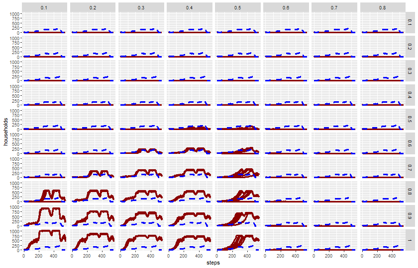

23.4 Use of machine learning for sensitivity analysis

To evaluate the importance of each parameter in a simulation model, Random Forest (RF) can be used as a feature importance estimator. This involves training an RF model on simulation results and then analyzing the impact of each input parameter on the output.

23.4.1 Step-by-Step Guide to Using Random Forest for Parameter Importance

1. Generate Simulation Data The first step is to generate simulation results by systematically sampling multiple parameters using methods like Random Sampling, Latin Hypercube Sampling (LHS), or Sobol Sampling.

Example: Generating Simulation Data in R

# Load required libraries
library(lhs)        # For Latin Hypercube Sampling
library(randtoolbox) # For Sobol Sampling

set.seed(123)
n <- 500  # Number of samples
k <- 5    # Number of parameters

# Generate Latin Hypercube sampled input parameters
param_samples <- randomLHS(n, k)
colnames(param_samples) <- paste0("param", 1:k)

# Assume a simple simulation model (e.g., sum of squared params)
simulation_results <- rowSums(param_samples^2)

# Convert to data frame
sim_data <- data.frame(param_samples, Output = simulation_results)

head(sim_data)

📌 Note: Replace simulation_results with the actual simulation output.

2. Train a Random Forest Model

Once the data is prepared, an RF model can be trained using randomForest in R.

Train the RF Model

library(randomForest)

# Train Random Forest to predict simulation output
set.seed(123)
rf_model <- randomForest(Output ~ ., data = sim_data, importance = TRUE, ntree = 500)

# Print model summary
print(rf_model)

📌 Explanation:

• Output ~ . means the RF model uses all parameters to predict the output.
  
• importance = TRUE ensures that feature importance is computed.
  
• ntree = 500 sets the number of trees in the forest.

3. Extract Parameter Importance

After training, RF provides two types of feature importance: 1. Mean Decrease in Accuracy (MDA) – Measures how much accuracy drops when a parameter is randomly shuffled. 2. Mean Decrease in Gini (MDG) – Measures how much each variable contributes to reducing node impurity in the decision trees.

Plot Feature Importance

# Extract importance values
importance_values <- importance(rf_model)

# Convert to a data frame
importance_df <- data.frame(Parameter = rownames(importance_values),
                            MDA = importance_values[, 1], 
                            MDG = importance_values[, 2])

# Print importance scores
print(importance_df)

# Plot feature importance
library(ggplot2)
ggplot(importance_df, aes(x = reorder(Parameter, -MDA), y = MDA)) +
  geom_bar(stat = "identity", fill = "steelblue") +
  labs(title = "Feature Importance (Mean Decrease in Accuracy)",
       x = "Parameter", y = "Importance") +
  theme_minimal()

📌 Interpretation: - Higher MDA values indicate more important parameters (greater accuracy drop when shuffled). - Higher MDG values mean stronger contributions to splitting decisions in trees.

4. Interpret the Results

After analyzing feature importance: - Key parameters can be identified for further refinement. - Unimportant parameters can be removed to simplify the model. - Interactions between parameters can be explored.

---

Summary | Step | Action | |——|——–| | 1 | Generate parameter samples using LHS, Sobol, or Random Sampling | | 2 | Run simulations to obtain output values | | 3 | Train a Random Forest model using randomForest | | 4 | Extract feature importance using importance() | | 5 | Interpret and visualize the results |

Example: (Angourakis et al. 2022)

23.5 Use of machine learning for parameter callibration

(TO-DO)

23.6 Use of machine learning for model selection

Example: (Carrignon, Brughmans, and Romanowska 2020)

Angourakis, Andreas, Jonas Alcaina-Mateos, Marco Madella, and Debora Zurro. 2022. “Human-Plant Coevolution: A Modelling Framework for Theory-Building on the Origins of Agriculture.” PLOS ONE 17 (9): e0260904. https://doi.org/10.1371/journal.pone.0260904.

Carrignon, Simon, Tom Brughmans, and Iza Romanowska. 2020. “Tableware Trade in the Roman East: Exploring Cultural and Economic Transmission with Agent-Based Modelling and Approximate Bayesian Computation.” Edited by Sergi Lozano. PLOS ONE 15 (11): e0240414. https://doi.org/10.1371/journal.pone.0240414.