6 Example: Settlement size, population and migration
6.1 Starting simple
As an example, let us imagine that in our research we postulate that:
the increase in the built-up area of an archaeological site, which we assumed to be a settlement, is explained by population growth due to migratory influx.
This general idea could be expressed more schematically as a set of cases or scenarios. Here we are limited to two:
↑ immigration → ↑ population → ↑ settlement size
↓ immigration → ↓ population → ↓ settlement size
We can also simplify this by sketching a causal diagram, a graph where the nodes are the “things” that change (the variables), the arrows mark the direction of the effect or causality, and their sign (+ or -), the sense of the effect (positive or negative):
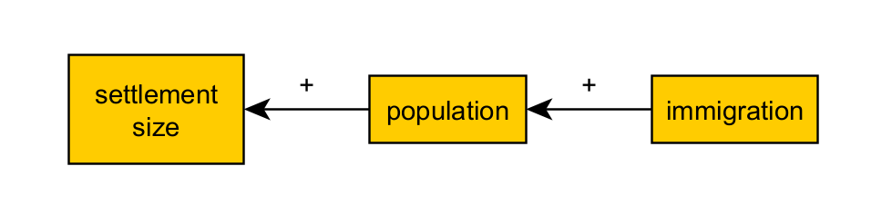
If we are comfortable with algebra, we could try to translate it to:
settlementSize = f(population) = f( g(immigration) )
or
settlementSize = f(population)
population = g(immigration)
where f and g are functions, yet to be defined.
what is a function?
a function is a relation between a set of inputs and a set of permissible outputs with the property that each input is related to exactly one output.
Such expressions rephrase the original explanation in a way that is more amenable to formalisation. They read as:
Settlement size (variable) is a function (depends on) population (variable).
Population (variable) is a function (depends on) immigration (variable).
Without equations to define f and g, our causal graph actually expresses more content by reading:
Settlement size (variable) is a function (depends on) population (variable) as a positive term (+).
Population (variable) is a function (depends on) immigration (variable) as a positive term (+).
6.2 Towards a balance between representation and complexity
Do you think this is a satisfactory description of our explanation? Does it leave out something we implicitly assumed with our first informal explanation? Is it going too far, stating something that we did not intend in the first place? The criteria for answering these questions push us away from the informal explanations and into the realm of logic and a broader contextual knowledge.
In our example, we can immediately detect that our variables must be expressed in at least two different units (e.g., \(m^{2}\) and individuals). We must add a parameter (a variable that remains constant throughout the process) to convert (amounts of) population into (amounts of) settlement size. We will call it areaPerInhabitant:
settlementSize = f(areaPerInhabitant * population)
Furthermore, we may find it insufficient to describe population change by considering only immigration (i.e., g(immigration)). You cannot tell how many apples are in a basket by just counting the ones you add. That is, we need an initial population:
population = g(initialPopulation, immigration)
Following the same reasoning, we should also consider that variables can change intrinsically (i.e., independently of g(immigration)) over time:
settlementSize = f(areaPerInhabitant * population, time)
population = g(initialPopulation, immigration, time)
If settlement size and population change over time, would immigration rates also change? If so, then we will also need to consider an additional term, the parameter that determines the rate of change in immigration:
settlementSize = f(population, time)
population = g(initialPopulation, immigration, time)
immigration = h(immigrationRate, time)
Our causal graph will be at this point considerably different, even when we assume time as implicit to all variables:
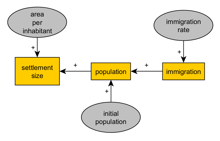
After a few iterations of this reasoning process, our formal expressions will undoubtedly become more complex. The more variables and parameters an explanatory model includes, the more realistic and rich the scenarios it will allow. However, variables and parameters should then be controlled by evidence or, at the very least, defined in a meaningful way.
Remember, while defining a parameter adds complexity, it also marks the point in a branch of thought where modelling stops, that is, where something that could certainly be described as complex and dynamic is reduced to a fixed value.
Important modelling terminology
Variable: it varies with time. It is part of the object of interest and its dynamics are interpreted as outputs of the phenomenon (≈model).
Parameter: it does not vary with time, but it can vary between instances of the phenomenon (≈simulation runs). It is considered as an input of the phenomenon (≈model).
In light of the context and research questions, you should decide when to sacrifice the representativeness of your model (the “want to”) to ensure that it can be implemented, understood, and validated in the future (the “can do”).
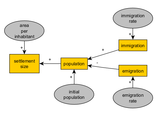
6.3 Reusing consolidated structures
When we are satisfied with a structure in our formalism, we can reuse it to extend the model and represent similar or symmetrical aspects of the phenomenon, without repeating the previous steps or making it less intelligible. For example, if our model considers immigration as a cause, we could also take into account an emigration flow with an opposite effect on the population.
6.4 Adding feedback loops
When representing processes, we must keep in mind that causality is not necessarily a unilateral relationship. Since we are considering the passage of time, a variable can be modelled to affect itself (in the future) or other variables that have previously influenced its value.
For example, given our background knowledge about population pressure, let’s stipulate that population positively affects the amount of emigration at a given time:
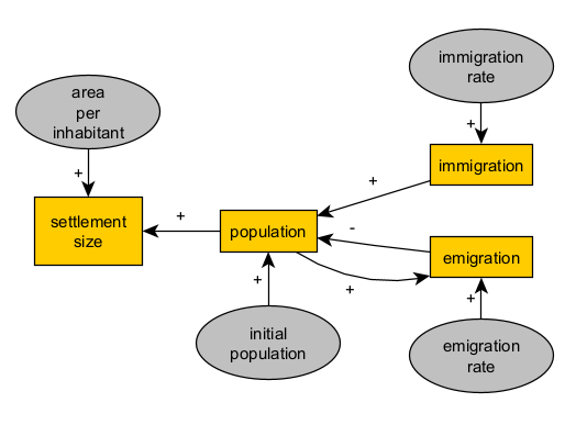
Reading:
>Population (variable) is a function (depends on) emigration (variable) as a negative term (-).
>Emigration (variable) is a function (depends on) population (variable) as a positive term (+).
With this idea, we can replace the parameter “initial population” with a positive loop (population-population), i.e., the initial population will simply be the value of population at the first time step. We can also improve our representation of how a real population by defining a component of the growth rate that is independent of migration flows (natural increase).
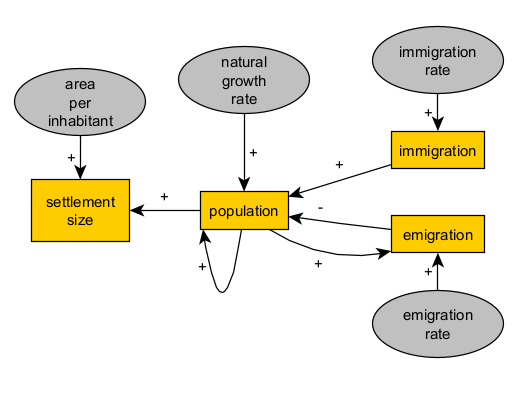
With this level of formalisation and complexity, our model will begin to approach a fully specified and implemented simulation model within the framework of system dynamics (https://en.wikipedia.org/wiki/System_dynamics). If we were to stay in this framework, we could already write down a preliminary implementation as a set of two difference equations:
population = naturalGrowthRate * population + immigrationRate - emmigrationRate * population
settlementSize = areaPerInhabitant * population
Through an examination of the causal diagram and the equations, we can visualise what aspects are detailed or simplified in our model. In this example, the model is clearly focusing more on population dynamics as the primary driver of settlement change, rather than other processes that could mediate population and settlement size (e.g., procurement of materials, construction, labour organisation, social norms of cohabitation). It is essential to decide whether this is desirable or not before continuing to add new elements to the model.
6.5 Expressing conditions as logic bifurcations
More often than not, explanations cannot be formalised solely with causal graphs and algebraic expressions like the ones above. One of the most common cases is when we want to represent a process that only occurs if certain conditions are met: a logical bifurcation or branching.
Imagine, for example, that our migration-driven population model must take into account the combined effect of two factors:
- The political relationship between this and neighbours (friendly/hostile)
- The general state of prosperity in the settlement (e.g. a combined factor of subsistence, well-being and raw material availability), summarised with a binary classification between good and bad times.
The introduction of the first factor can be simple: a hostile relationship will prevent any migration flow, incoming or outgoing. The corresponding diagram, now expressed as a flowchart, could be:
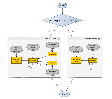
Note: the logic bifurcations are not part of the causal graph. They are part of the model’s logic.
The second factor will create yet another bifurcation, relevant only if the settlement’s neighborhood is friendly. If times are good, we will assume that immigration is triggered, because the settlement is attractive to new residents. If times are bad, emigration is triggered instead, to represent the growing number of inhabitants who are dissatisfied with local living conditions.
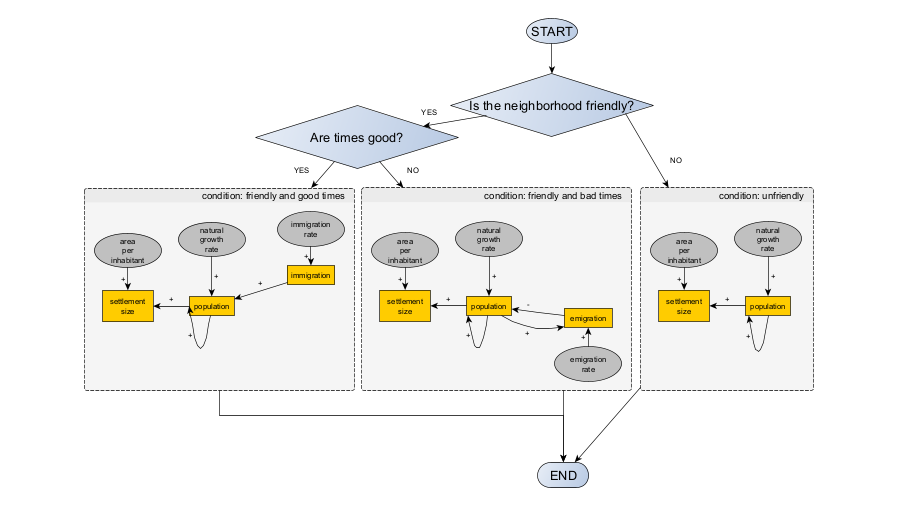
The more your formal model is composed of algorithms (discontinuous operations) rather than equations (continuous operations), the more complicated it will be to use causal diagrams and the easier it will be to use of flowcharts and other specialised diagrams (e.g. UML). However, when it comes to model development and communication, ANY diagram is better than NO diagram or conceptual formalism at all.
6.6 Representing distributed and social mechanisms
If we are looking for a formal model capable of accounting for distributed processes (occurring in parallel through the action of multiple entities) and more complex social mechanisms (i.e. multi-dimensional, non-linear), our conceptual model should move towards an object-based and, eventually, agent-based framework. There are many ways to represent distributed processes, such as formulating variables as vectors and matrices, if equations are still a viable format, or drawing flowcharts to prescribe the behaviour of entities and their potential interactions.
If our population model were to be formulated as agent-based, considering households as the primary units of the process, we would need to define their behaviour in a way that, in aggregate, still represents the essence of the causal relationship we seek to formalise:
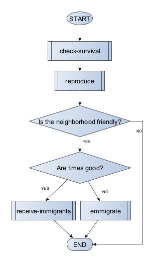
Notice that once the process is conceptualised as distributed, it will be increasingly more challenging to keep the description of the conceptual model in a single formal expression or diagram. In the example above, we choose to simplify the diagram by referencing entire chunks of our model by a single meaningful name (e.g., “reproduce”). These named chunks are the best candidates to be implemented later on as functions: a bundle of operations that can take inputs and return outputs.
For example, let us define “reproduce” as a decision on whether a household will branch a new one given that a certain probability threshold, called the household fission rate, a household-level parameter replacing the population-level natural growth rate:
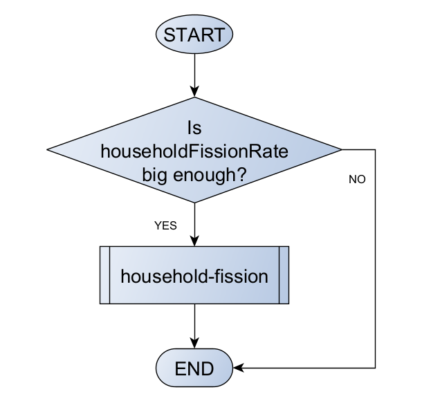
Remember, specifications can be at this stage still quite vague and undefined. For example, how should we determine whether the household fission rate is sufficiently large? Moreover, observe how, yet again, we rely on the promise of a new function, household fission. Thinking of functions in terms of modules can help us expand our conceptual model without getting stuck on details that will only be truly handled once we move to implementation.